AMS机器学习课程:Keras深度学习 - 人工神经网络
本文翻译自 AMS 机器学习 Python 教程,并有部分修改。
David John Gagne, 2019: “Deep Learning with Keras”.
https://github.com/djgagne/ams-ml-python-course/blob/master/module_3/ML_Short_Course_Module_3_Deep_Learning.ipynb
David John Gagne, National Center for Atmospheric Research
介绍
目标
了解深度学习的定义及其与传统机器学习方法的区别
了解 Keras 是什么,它如何工作以及如何与其他深度学习库交互
在 Keras 中建立一个全连接神经网络
了解激活函数的选择如何影响性能
在 Keras 中建立卷积神经网络,并与全连接神经网络比较,看看它的性能如何
了解数据是如何通过卷积层转换的
软件需求
本节使用如下的软件库
Python 3.6 或更高版本
Numpy
Pandas
Matplotlib
IPython
Jupyter
Xarray
netCDF4
Tensorflow (为训练卷积神经网络,推荐使用 GPU 版本)
Keras
CUDA 9.2 或更高版本和 cuDNN (用于与 NVIDIA GPU 接口)
什么是深度学习

深度学习应在人工智能和机器学习的背景下进行定义。
人工智能 (Artificial Intelligence, AI):计算机执行传统上由人类完成的认知任务而无需人类直接控制的多种方式。
从历史上看,开发人工智能系统有两种思想流派。
专家系统 (Expert Systems):任务专家创建描述任务完成方式的算法和规则,然后 AI 程序根据规则完成任务。
通常实现为模糊逻辑 (Fuzzy Logic)
业务示例:NEXRAD Hydrometeor 分类算法,基于对象的诊断评估方法 (Method for Object-based Diagnostic Evaluation, MODE)
优点:不需要数据,可解释,可控制
缺点:算法脆弱,复杂性难以管理,无法自适应
机器学习 (Machine Learning, ML):具有指定结构的数学模型,从数据中学习执行任务
常用算法:神经网络 (Neural networks),决策树 (Decision trees),支持向量机 (Support vector machines)
优点:具有较高的预测能力,可以学习复杂的模式和关系,量化不确定性,可以解释
缺点:需要大量数据,特征的大量预处理,外推问题
深度学习 (Deep Learning):机器学习的一个子集,由神经网络和许多专门的隐藏层组成,用于对输入数据中的结构模式进行编码以产生更好的预测
常用算法:卷积神经网络 (Convolutional neural networks),递归神经网络 (Recurrent neural networks)
优点:与传统机器学习相比,在图像和时序问题上的预测能力更高,所需的预处理和特征提取更少
缺点:比传统机器学习需要更多的数据和计算资源,更难于训练,对对抗性数据的敏感性更高
什么是 Keras
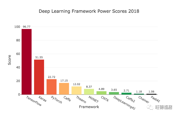
Keras 是用于深度学习的以人为本的高级API。Keras 提供了一个面向对象的接口,用于通过以不同方式将各层连接在一起来创建任意复杂度的神经网络。因为 Keras 旨在成为一个接口,而不是一个完整的深度学习库,所以它已在多个深度学习库和其他编程语言的基础上实现。Keras 充当 Tensorflow 的官方高级 API,并且还可以与 Theano 和 Microsoft 的 CNTK 交互。Keras 还有一个 R 接口。
Keras 使用分层对象表示神经网络。完整的网络存储为 Model 对象,其中包含可顺序或任意连接的层列表。每个层都是其自己的对象,并包含名称和参数,包括权重和配置。为了进行训练和推理,Keras 实现了 scikit-learn 的 fit 和 perdict API,还提供了调用模型及其单个组件的低级方法。keras 后端提供了通过模型的任意子集传递数据的方法,这将使我们能够看到神经网络如何转换数据以进行预测。
数据
本文数据的下载方法请查阅
准备
载入需要使用的库
import numpy as np
import pandas as pd
import xarray as xr
import matplotlib.pyplot as plt

import pathlib
from tqdm.notebook import tqdm
载入
首先,我们将加载训练网络所需的 csv 数据文件并将它们连接在一起。
csv_path = pathlib.Path("../data/track_data_ncar_ams_3km_csv_small")
csv_files = sorted(csv_path.glob("*.csv"))
len(csv_files)
100
使用 pd.read_csv() 加载 CSV 文件
csv_data_list = []
for csv_file in csv_files:
    csv_data_list.append(pd.read_csv(csv_file))
使用 pd.concat 将多个 DataFrame 对象合并为一个对象。同时删掉列表对象以节省空间
csv_data = pd.concat(csv_data_list, ignore_index=True)
del csv_data_list
CSV 数据文件中的列名
for column in csv_data.columns:
    print(column)
Step_ID
Track_ID
Ensemble_Name
Ensemble_Member
Run_Date
Valid_Date
Forecast_Hour
Valid_Hour_UTC
Duration
Centroid_Lon
Centroid_Lat
Centroid_X
Centroid_Y
Storm_Motion_U
Storm_Motion_V
REFL_COM_mean
REFL_COM_max
REFL_COM_min
REFL_COM_std
REFL_COM_percentile_10
REFL_COM_percentile_25
REFL_COM_percentile_50
REFL_COM_percentile_75
REFL_COM_percentile_90
U10_mean
U10_max
U10_min
U10_std
U10_percentile_10
U10_percentile_25
U10_percentile_50
U10_percentile_75
U10_percentile_90
V10_mean
V10_max
V10_min
V10_std
V10_percentile_10
V10_percentile_25
V10_percentile_50
V10_percentile_75
V10_percentile_90
T2_mean
T2_max
T2_min
T2_std
T2_percentile_10
T2_percentile_25
T2_percentile_50
T2_percentile_75
T2_percentile_90
RVORT1_MAX-future_mean
RVORT1_MAX-future_max
RVORT1_MAX-future_min
RVORT1_MAX-future_std
RVORT1_MAX-future_percentile_10
RVORT1_MAX-future_percentile_25
RVORT1_MAX-future_percentile_50
RVORT1_MAX-future_percentile_75
RVORT1_MAX-future_percentile_90
HAIL_MAXK1-future_mean
HAIL_MAXK1-future_max
HAIL_MAXK1-future_min
HAIL_MAXK1-future_std
HAIL_MAXK1-future_percentile_10
HAIL_MAXK1-future_percentile_25
HAIL_MAXK1-future_percentile_50
HAIL_MAXK1-future_percentile_75
HAIL_MAXK1-future_percentile_90
area
eccentricity
major_axis_length
minor_axis_length
orientation
Matched
Max_Hail_Size
Num_Matches
Shape
Location
Scale
问题
我们将选择一组输入变量和一个输出字段,根据日期拆分数据,并提取强旋转 (strong rotation) 情况。
定义问题
输入和输出变量
input_columns = [
    "REFL_COM_mean",
    "U10_mean",
    "V10_mean",
    "T2_mean"
]

output_column = "RVORT1_MAX-future_max"
涡度阈值,s-1。
使用阈值将连续数据变为离散数据,从而形成分类问题
out_threshold = 0.005构建训练集和测试集
将数据集按时间分为训练集和测试集
train_test_date = pd.Timestamp("2015-01-01")使用 Valid_Date 字段筛选
valid_dates = pd.DatetimeIndex(csv_data["Valid_Date"])
valid_dates
DatetimeIndex(['2010-10-24 12:00:00', '2010-10-24 12:00:00',
'2010-10-24 12:00:00', '2010-10-24 13:00:00',
'2010-10-24 14:00:00', '2010-10-24 15:00:00',
'2010-10-24 12:00:00', '2010-10-24 13:00:00',
'2010-10-24 14:00:00', '2010-10-24 15:00:00',
...
'2017-03-30 11:00:00', '2017-03-30 11:00:00',
'2017-03-30 11:00:00', '2017-03-30 11:00:00',
'2017-03-30 11:00:00', '2017-03-30 11:00:00',
'2017-03-30 11:00:00', '2017-03-30 11:00:00',
'2017-03-30 11:00:00', '2017-03-30 11:00:00'],
dtype='datetime64[ns]', name='Valid_Date', length=121137, freq=None)
为神经网络提取训练输入数据
train_data = csv_data.loc[valid_dates < train_test_date, input_columns]
train_data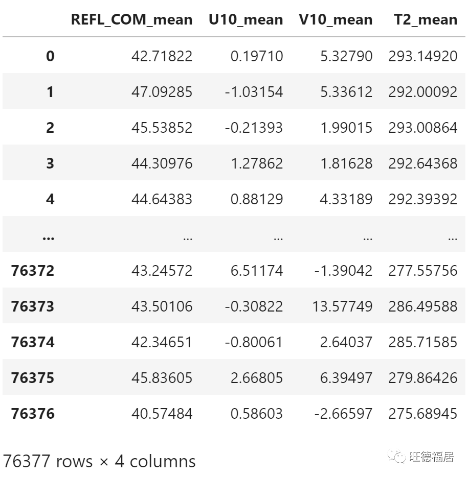
提取训练目标数据,将强旋转标记为 1,弱旋转或无旋转标记为 0
train_out = np.where(
    csv_data.loc[valid_dates < train_test_date, output_column] > out_threshold,
    1,
    0,
)
train_out
array([0, 0, 0, ..., 0, 0, 0])
训练数据中强旋转的比例
train_out.sum() / train_out.size * 1004.552417612632075
提取测试数据
test_data = csv_data.loc[valid_dates >= train_test_date, input_columns]
test_data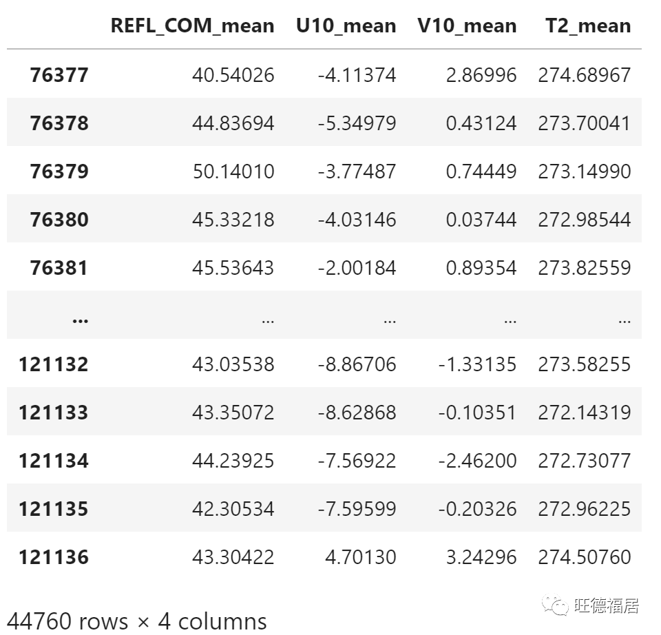
test_out = np.where(
    csv_data.loc[valid_dates >= train_test_date, output_column] > out_threshold,
    1,
    0,
)
测试数据中强旋转的比例
test_out.sum() / test_out.size * 1005.26586237712243
处理输入数据
我们将使用标准缩放器对神经网络的输入数据进行归一化。
用训练集适配归一化器 StandardScaler
from sklearn.preprocessing import StandardScaler

scaler = StandardScaler()
train_norm = scaler.fit_transform(train_data)
每个输入变量的归一化参数
for i, input_col in enumerate(input_columns):
    print(
        f"{input_columns[i]:13s} "
        f"Mean: {scaler.mean_[i]:.3f} "
        f"SD: {scaler.scale_[i]:.3f}"
    )
REFL_COM_mean Mean: 46.847 SD: 3.984
U10_mean Mean: 0.450 SD: 4.348
V10_mean Mean: 0.543 SD: 4.462
T2_mean Mean: 289.409 SD: 6.932
使用训练集的归一化参数处理测试数据
test_norm = scaler.transform(test_data)方法
Dense Neural Networks 稠密神经网络
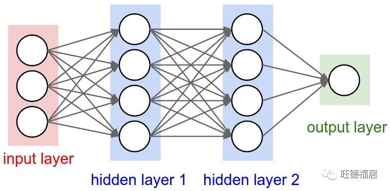
人工神经网络 (Artificial neural network) 是一种机器学习算法,可以将一组输入非线性转换为一个或多个输出。人工神经网络受到大脑中神经元的工作方式的模糊启发,但并未明确地对大脑建模。神经网络由一个输入层,一个或多个隐藏层以及一个输出层组成。隐藏层对上一层的输出执行转换,输出层将隐藏表示转换为预测。每层由一组感知器 (perceptrons) 或人工神经元 (artificial neurons) 组成。
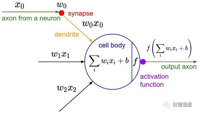
在每个神经元内部是一组与神经元的每个输入关联的权重和一个附加偏差项。本质上,这部分是线性回归。输入乘以权重,然后相加。
激活函数
然后,该总和通过激活函数 (activation function) 传递,该函数以某种非线性方式转换数据。激活函数的目标通常是通过将某些神经元设置为 0 来增加表示的稀疏性或限制可能值的范围。通常在网络的密集层或卷积层之后直接使用激活。下面绘制了一组常见的激活函数及其梯度或导数。
占位符输入张量允许将 numpy 数组通过函数馈入 Tensorflow
译者注:因为安装的 tensorflow 版本是 2.x,这里使用兼容 v1 版本的接口
import tensorflow as tf
import tensorflow.compat.v1.keras as keras
import tensorflow.compat.v1.keras.backend as K

config = tf.compat.v1.ConfigProto()
config.gpu_options.allow_growth = True
session = tf.compat.v1.Session(config=config)
K.set_session(session)

tf.compat.v1.disable_eager_execution()

act_in = K.placeholder()
激活函数列表
activations = [
    "sigmoid",
    "tanh",
    "relu",
    "elu",
]
准备数据对象
from tensorflow.compat.v1.keras.layers import Activation, LeakyReLU

input_vals = np.linspace(-2, 2, 100)
output_vals = []

activation_functions = []
绘图
K.function 在 2 个相连的 keras 张量之间创建通用输入输出函数
K.gradients 计算任意输入和输出配对之间的梯度
plt.figure(figsize=(12, 6))

# 函数值
plt.subplot(1, 2, 1)
plt.plot(
    input_vals,
    np.zeros(input_vals.shape),
    "k--"
)

for activation in activations:
    activation_functions.append(
        K.function(
            [act_in],
            [Activation(activation)(act_in)]
        )
    )

    output_vals.append(activation_functions[-1]([input_vals])[0])

    plt.plot(
        input_vals,
        output_vals[-1],
        label=activation,
    )

activation_functions.append(
    K.function(
        [act_in],
        [LeakyReLU(0.2)(act_in)]
    )
)
output_vals.append(
    activation_functions[-1]([input_vals])[0]
)
plt.plot(
    input_vals,
    output_vals[-1],
    label="leaky relu",
)

plt.xlabel("Input", fontsize=14)
plt.ylabel("Activation", fontsize=14)
plt.title("ANN Ativation Functions", fontsize=16)
plt.legend(fontsize=12)

# 梯度
plt.subplot(1, 2, 2)
plt.plot(
    input_vals,
    np.zeros(input_vals.shape),
    "k--",
)
for activation in activations:
    activation_functions.append(
        K.function(
            [act_in],
            K.gradients(Activation(activation)(act_in), act_in)
        )
    )
    output_vals.append(activation_functions[-1]([input_vals])[0])
    plt.plot(
        input_vals,
        output_vals[-1],
        label=activation
    )

activation_functions.append(
    K.function(
        [act_in],
        K.gradients(LeakyReLU(0.2)(act_in), act_in)
    )
)
output_vals.append(
    activation_functions[-1]([input_vals])[0]
)
plt.plot(
    input_vals,
    output_vals[-1],
    label="leaky relu",
)

plt.xlabel("Input", fontsize=14)
plt.ylabel("Activation Gradients", fontsize=14)
plt.title("Ann Activation Gradients", fontsize=16)
plt.show()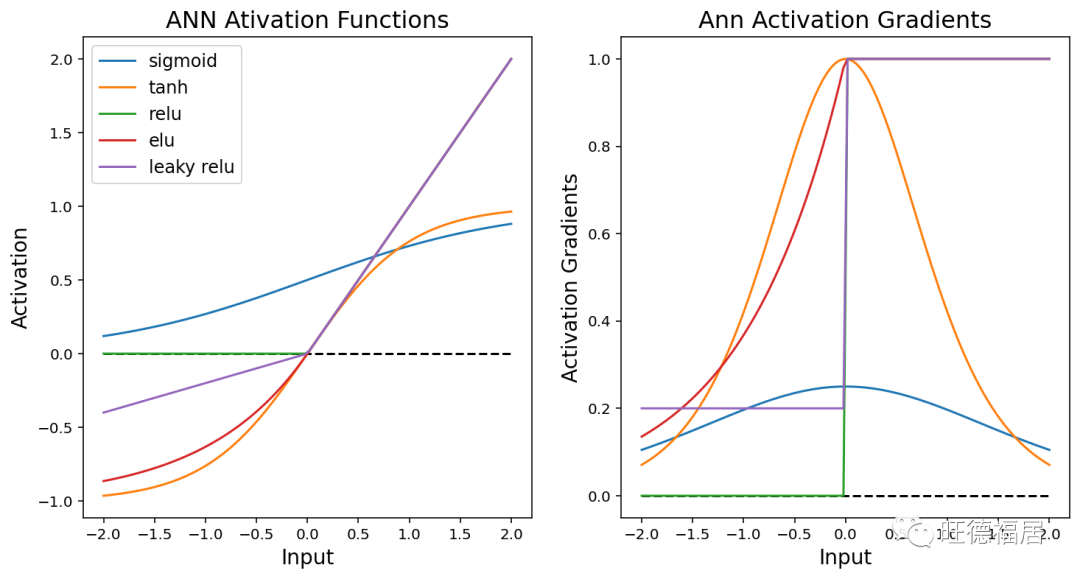
常见的激活函数如上图所示。传统的人工神经网络使用 sigmoid 或双曲线正切(tanh)激活函数来模拟大脑中神经元的激活。sigmoids 和 tanh 的问题在于,当错误信息通过网络反向传播时,sigmoids 的最大斜率(相对于输出变化的输入导数)约为 0.3,因此每次向后通过 sigmoids 将梯度幅度降低 70% 或更多。这导致了深度神经网络的“消失梯度问题 (vanishing gradient problem)”。在 2 或 3 层之后,梯度的大小太小,无法提供有关权重如何更新的一致信号,从而导致模型的收敛性较差。
Rectified Linear Unit (ReLU) 激活通过执行变换来解决此问题,即正值保留其原始大小而负值设置为0。由于正梯度的大小不会减小,因此梯度信号可以传播很多层而不消失。将负梯度清零有时可能会导致神经元死亡,因此已创建 ReLU 的变体(例如 Leaky ReLU 和 Exponential Linear Unit (ELU))来传播负信息,但幅度减小。
神经网络训练
通过随机梯度下降 (stochastic gradient descent) 过程优化神经网络的权重。
一批或随机的训练数据子集通过神经网络发送以生成预测。
通过使用损失或误差函数,将这些预测与真实的标签或值进行比较。回归的常见误差函数是均方误差 (Mean squared error)。由于均方误差等于 Brier 评分 (Brier Score),因此它也可以用于二元分类问题。分类的另一个常见损失函数是交叉熵 (cross-entropy),即
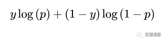
其中 y 为 1 或 0,而 p 为预测概率。
计算出相对于网络中每个权重的误差的导数(dL/dw)。网络中给定权重的导数取决于给定神经元和输出层之间任何神经元的权重的导数,因此必须首先计算这些导数。此过程称为反向传播 (back-propagation)。
一旦为给定的权重计算了导数,就通过从原始权重中减去导数的一部分来更新权重。
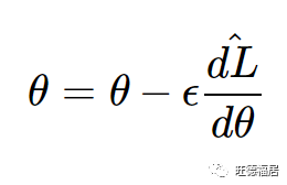
分数 theta 被称为学习率。通过逆梯度进行优化的过程称为梯度下降 (gradient descent)。当对训练数据的随机子集而不是所有训练数据执行时,该过程称为随机梯度下降 (stochastic gradient descent)。
较大的学习速率会导致更快的收敛速度,但是太大的学习速率会导致优化器超出全局最小值。如果学习率太小,则优化器可能会陷入局部最小值或永远不会收敛。已经开发出专门的优化器功能来解决其中一些问题。
SGD:Stochastic Gradient Descent,随机梯度下降。随机成分来自为每个更新选择随机的训练示例“批次”。SGD 包括一个向梯度下降更新添加动量的选项,该选项使优化器可以保留以前的梯度在随机梯度计算中减少方差的记忆。实际上,通常建议在 0.99 附近使用较高的动量值。
Adam:“adaptive moment”的缩写。该优化器根据 first and second moments of the gradient 自动更新学习率。关键参数是 beta_1 和 beta_2,分别默认为 0.9 和 0.99。作者已经成功地将学习率和 beta_1 设置为较低的值,但是默认值效果很好。
实现
Keras 稠密神经网络
现在我们训练一个简单的单层神经网络,预测强旋转的概率
注:这里的单层指的是只有一个隐藏层
配置
设置块大小
batch_size = 128一个 epoch 是对训练数据的一次遍历
num_epochs = 10隐藏层中的神经元数目
hidden_neurons = 10学习率
learning_rate = 0.01使用 SGD 优化器,或将其修改为 Adam 对象
from tensorflow.compat.v1.keras.optimizers import SGD, Adam

optimizer = SGD(
    lr=learning_rate,
    momentum=0.9,
)
损失函数可以是 binary_crossentropy 或者 mse
loss = "binary_crossentropy"构建网络
创建输入层
from tensorflow.compat.v1.keras.layers import Input

small_net_input = Input(
    shape=(len(input_columns),)
)
small_net_input
<tf.Tensor 'input_1:0' shape=(None, 4) dtype=float32>
隐藏层,使用 tanh 激活函数
from tensorflow.compat.v1.keras.layers import Dense

small_net_hidden = Dense(
    hidden_neurons,
    activation="tanh"
)(small_net_input)
small_net_hidden
<tf.Tensor 'dense/Tanh:0' shape=(None, 10) dtype=float32>
输出层,使用 sigmoid 激活函数
small_net_out = Dense(
    1,
    activation="sigmoid"
)(small_net_hidden)
small_net_out
<tf.Tensor 'dense_1/Sigmoid:0' shape=(None, 1) dtype=float32>
将上面层合并为一个模型对象
from tensorflow.compat.v1.keras.models import Model

small_model = Model(
    small_net_input,
    small_net_out,
)
small_model
<tensorflow.python.keras.engine.functional.Functional at 0x1b33dce63c8>
编译模型对象,实例化所有的 tensorflow 连接
small_model.compile(
    optimizer,
    loss=loss,
)
训练
块大小 batch_size 应该能整除训练样本数。将剩余样本去除以确保这点。
batch_diff = train_norm.shape[0] % batch_size创建训练集索引,为后续随机块采样做准备
batch_indices = np.arange(train_norm.shape[0] - batch_diff)
num_batches = int(batch_indices.size / batch_size)
从网络中提取权重
hw:hidden weights,隐藏层权重,(4, 10),即将 4 个输入变量映射到 10 个单元中hb:hidden biasow:output weights,输出层权重,(10, 1),即将 10 个变量映射到 1 个单元中ob:output bias
hw, hb, ow, ob = small_model.get_weights()
hw.shape, ow.shape
((4, 10), (10, 1))
为每块保存隐藏和输出层的权重
hw_series = np.zeros(
    [num_batches * num_epochs] + list(hw.shape)
)
ow_series = np.zeros(
    [num_batches * num_epochs] + list(ow.shape)
)
hw_series.shape
(5960, 4, 10)
迭代训练
i = 0
for e in tqdm(range(num_epochs)):
    # 每个 epoch 开始,洗牌训练样本
    batch_indices = np.random.permutation(batch_indices)
    for b in range(num_batches):
        hw_series[i], hb, ow_series[i], ob = small_model.get_weights()
        # 根据一块训练数据执行一次更新
        small_model.train_on_batch(
            train_norm[batch_indices[b * batch_size: (b+1) * batch_size]],
            train_out[batch_indices[b * batch_size: (b+1) * batch_size]],
        )
        i = i + 1
下面是我们刚训练的神经网络模型的汇总信息
small_model.summary()Model: "functional_1"
_________________________________________________________________
Layer (type) Output Shape Param #
=================================================================
input_1 (InputLayer) [(None, 4)] 0
_________________________________________________________________
dense (Dense) (None, 10) 50
_________________________________________________________________
dense_1 (Dense) (None, 1) 11
=================================================================
Total params: 61
Trainable params: 61
Non-trainable params: 0
_________________________________________________________________
神经网络权重的演变
现在我们将绘制神经网络权重的变化图。请注意,所有权重是如何在随机位置开始的,但是有些权重会随着时间发生显着变化。返回并以不同的学习率或批次大小重新训练网络。这如何改变权重的轨迹?
fig = plt.figure(figsize=(12, 5))
plt.subplot(1, 2, 1)

hw_flat = hw_series.reshape(
    hw_series.shape[0],
    hw_series.shape[1] * hw_series.shape[2]
)

for i in range(hw_flat.shape[1]):
    plt.plot(hw_flat[:, i])
plt.xlabel("Step", fontsize=14)
plt.ylabel("Weight", fontsize=14)
plt.title("Hidden Layer Weights Optimized")

plt.subplot(1, 2, 2)
ow_flat = ow_series.reshape(
    ow_series.shape[0],
    ow_series.shape[1] * ow_series.shape[2]
)

for i in range(ow_flat.shape[1]):
    plt.plot(ow_flat[:, i])
plt.xlabel("Step", fontsize=14)
plt.ylabel("Weight", fontsize=14)
plt.title("Output Layer Weights Optimized")
plt.show()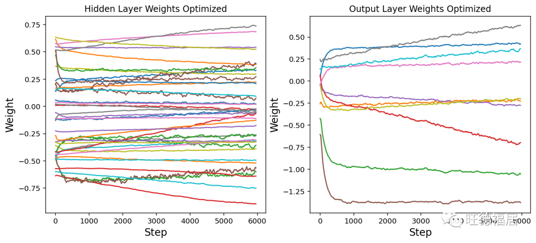
我们还可以通过调用 fit 方法并指定时期数和批量大小来训练神经网络。
small_model.fit(
    train_norm,
    train_out,
    epochs=10,
    batch_size=128,
)
结果
稠密神经网络检验
现在,我们将计算一些检验分数,以确定神经网络的性能。我们将使用 3 个常见的摘要分数:
Area Under the ROC Curve (AUC):衡量模型在两个类别之间的区分程度,或最小化 false alarms 和 true negatives 的数量。
Brier Score:概率预测的均方误差。测量辨别力 (discrimination),可靠性 (reliability) 和清晰度 (sharpness) 的组合。
Brier Skill Score:与始终按给定事件的观测相对频率进行预测相比,概率预测提高的百分比。
预测测试集
from sklearn.metrics import (
    mean_squared_error,
    roc_auc_score
)

small_model_preds = small_model.predict(test_norm).ravel()
small_model_preds
array([0.00285614, 0.0076969 , 0.05562624, ..., 0.00773937, 0.00463793,
0.00454199], dtype=float32)
AUC
small_model_auc = roc_auc_score(test_out, small_model_preds)
small_model_auc
0.8876840181625545
Brier Score
small_model_brier_score = mean_squared_error(test_out, small_model_preds)
small_model_brier_score
0.03896855574047458
Brier Skill Score
climo_brier_score = mean_squared_error(
    test_out,
    np.ones(test_out.size) * test_out.sum() / test_out.size
)

small_model_brier_skill_score = 1 - small_model_brier_score / climo_brier_score
small_model_brier_skill_score
0.21884305282434524
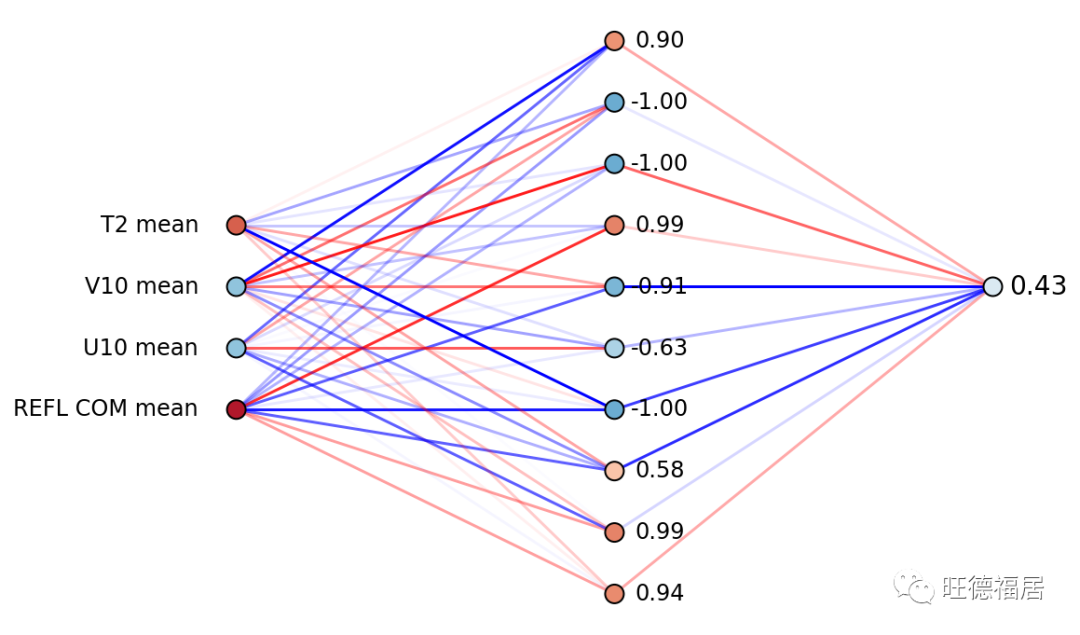
神经网络内部可视化
数据通过神经网络时会发生什么变化?
下面是给定一组输入字段的神经网络内部的静态和交互式可视化。彩色圆圈表示特定神经元的值。红色为正,蓝色为负。彩色线显示分配给每个连接的权重。深色线条的权重较大。
def plot_neural_net(
neural_net,
refl,
u10,
v10,
t2
):
plt.figure(figsize=(8, 6))
# 值
nn_func = K.function(
[neural_net.input],
[
neural_net.layers[1].output,
neural_net.layers[2].output,
]
)
h1_out, out_out = nn_func(
[np.array([[refl, u10, v10, t2]])]
)
# 权重
h_weights = neural_net.layers[1].get_weights()[0]
out_weights = neural_net.layers[2].get_weights()[0]
plt.axis("off")
i1 = 0
for y1 in range(3, 7):
# 输入层:变量名
plt.text(
-0.1, y1,
input_columns[i1].replace("_", " "),
ha='right',
va='center',
fontsize=12
)
# 输入层 -> 隐藏层:权重
for y2 in range(0, 10):
if h_weights[i1, y2] > 0:
color = [1, 0, 0, np.abs(h_weights[i1, y2]) / np.abs(h_weights).max()]
else:
color = [0, 0, 1, np.abs(h_weights[i1, y2]) / np.abs(h_weights).max()]
plt.plot(
[0, 1], [y1, y2],
linestyle='-',
color=color,
zorder=0
)
i1 += 1
# 隐藏层 -> 输出层:权重
for y2 in range(0, 10):
if out_weights[y2, 0] > 0:
color = (1, 0, 0, np.abs(out_weights[y2, 0] / np.abs(out_weights).max()))
else:
color = (0, 0, 1, np.abs(out_weights[y2, 0] / np.abs(out_weights).max()))
plt.plot(
[1, 2], [y2, 5],
linestyle='-',
color=color,
zorder=0
)
# 输入层:散点
plt.scatter(
np.zeros(4),
np.arange(3, 7),
100,
np.array([refl, u10, v10, t2]),
vmin=-5,
vmax=5,
cmap="RdBu_r",
edgecolor='k',
)
# 隐藏层:散点
plt.scatter(
np.ones(h1_out.size),
np.arange(h1_out.size),
100,
h1_out.ravel(),
edgecolor='k',
vmin=-2,
vmax=2,
cmap="RdBu_r"
)
# 隐藏层:值
for i in range(10):
plt.text(
1.12, i,
"{0:0.2f}".format(h1_out.ravel()[i]),
ha='center',
va='center',
fontsize=12
)
# 输出层:散点
plt.scatter(
[2],
[5],
[100],
out_out[0],
vmin=0,
vmax=1,
cmap="RdBu_r",
edgecolor='k'
)
# 输出层:值
plt.text(
2.12, 5,"{0:0.2f}".format(out_out[0, 0]),
ha='center',
va='center',
fontsize=14
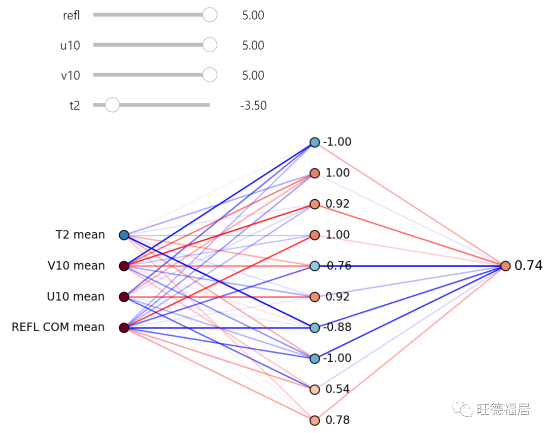
)示例
plot_neural_net(
    small_model,
    refl=4,
    u10=-2,
    v10=-2,
    t2=3
)
移动滑块以更改输出值。看看是否可以最大化强旋转的可能性。
from ipywidgets import interact
import ipywidgets as widgets

interact(
    lambda refl, u10, v10, t2: plot_neural_net(small_model, refl, u10, v10, t2),
    refl=widgets.FloatSlider(min=-5, max=5, step=0.1),
    u10=widgets.FloatSlider(min=-5, max=5, step=0.1),
    v10=widgets.FloatSlider(min=-5, max=5, step=0.1),
    t2=widgets.FloatSlider(min=-5, max=5, step=0.1)
);
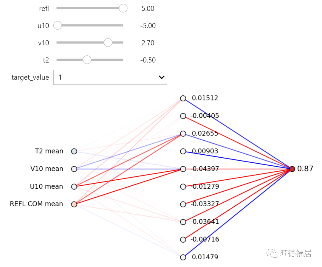
神经网络梯度可视化
当一组输入通过网络时,我们还可以绘制神经网络权重和值的梯度。将目标值从 0 更改为 1 时,梯度如何变化?改变每个输入字段如何影响整个网络的梯度?
def plot_gradient(
    neural_net,
    refl,
    u10,
    v10,
    t2,
    target_value,
):
    plt.figure(figsize=(8, 6))
    nn_func = K.function(
        [neural_net.input],
        [
            neural_net.layers[1].output,
            neural_net.layers[2].output
        ]
    )

    target = K.placeholder(shape=(1,))
    loss = K.mean((neural_net.output - target) ** 2)
    grads = K.gradients(
        loss,
        neural_net.layers[1].weights + neural_net.layers[2].weights +
        [neural_net.layers[1].output, neural_net.input]
    )

    grad_func = K.function(
        [neural_net.input, target],
        grads
    )

    # 值
    h1_out, out_out = nn_func(
        [np.array([[refl, u10, v10, t2]])]
    )

    # 梯度
    (
        hidden_weight_grad,
        hidden_bias_grad,
        out_weight_grad,
        out_bias_grad,
        hidden_grad,
        input_grad,
    ) = grad_func(
        [
            np.array([[refl, u10, v10, t2]]),
            np.array([target_value])
        ]
    )

    # 权重
    h_weights = neural_net.layers[1].get_weights()[0]
    out_weights = neural_net.layers[2].get_weights()[0]

    plt.axis("off")

    i1 = 0
    for y1 in range(3, 7):
        plt.text(
            -0.1, y1,
            input_columns[i1].replace("_", " "),
            ha='right',
            va='center',
            fontsize=12
        )
        for y2 in range(0, 10):
            if h_weights[i1, y2] < 0:
                color = [
                    1, 0, 0,
                    np.abs(hidden_weight_grad[i1, y2]) / np.abs(hidden_weight_grad).max()
                ]
            else:
                color = [
                    0, 0, 1,
                    np.abs(hidden_weight_grad[i1, y2]) / np.abs(hidden_weight_grad).max()
                ]
            plt.plot(
                [0, 1], [y1, y2],
                linestyle='-',
                color=color,
                zorder=0
            )
        i1 += 1

    for y2 in range(0, 10):
        if out_weights[y2, 0] < 0:
            color = (
                1, 0, 0,
                np.abs(out_weight_grad[y2, 0] / np.abs(out_weight_grad).max())
            )
        else:
            color = (
                0, 0, 1,
                np.abs(out_weight_grad[y2, 0] / np.abs(out_weight_grad).max())
            )
        plt.plot(
            [1, 2], [y2, 5],
            linestyle='-',
            color=color,
            zorder=0
        )

    plt.scatter(
        np.zeros(4), np.arange(3, 7), 100,
        -input_grad.ravel() / np.abs(input_grad).max(),
        vmin=-5,
        vmax=5,
        cmap="RdBu_r",
        edgecolor='k',
    )

    plt.scatter(
        np.ones(h1_out.size), np.arange(h1_out.size), 100,
        -hidden_grad.ravel(),
        edgecolor='k',
        vmin=-2,
        vmax=2,
        cmap="RdBu_r"
    )

    for i in range(10):
        plt.text(
            1.2, i,
            "{0:0.5f}".format(-hidden_grad.ravel()[i]),
            ha='center',
            va='center',
            fontsize=12
        )
    plt.scatter(
        [2], [5], [100],
        out_out[0],
        vmin=0,
        vmax=1,
        cmap="RdBu_r",
        edgecolor='k'
    )

    plt.text(
        2.12, 5,
        "{0:0.2f}".format(out_out[0, 0]),
        ha='center',
        va='center',
        fontsize=14
    )
interact(
lambda refl, u10, v10, t2, target_value:
plot_gradient(
small_model, refl, u10, v10, t2, target_value
),
refl=widgets.FloatSlider(value=1.0, min=-5, max=5, step=0.1),
u10=widgets.FloatSlider(value=-1.0,min=-5, max=5, step=0.1),
v10=widgets.FloatSlider(value=1.0, min=-5, max=5, step=0.1),
t2=widgets.FloatSlider(value=1.0, min=-5, max=5, step=0.1),
target_value=[0, 1]
);
参考
https://github.com/djgagne/ams-ml-python-course
AMS 机器学习课程
数据预处理:
实际数据处理:
线性回归:
逻辑回归:
决策树: